
One of the first things that you learn when you start studying statistics is the normal distribution which is also known as the Gaussian distribution or normal bell curve.
Discover the z tables you need here.

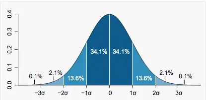
As you can see from the image above, the normal distribution tapers out in both tails and is dense in the middle.
Imagine that a teacher wants to create a curve based on the exam scores. This means that he will be fitting the scores to the bell curve. When he is filling the chart, the grades will be centered around the mean score (the tallest, central point on the curve, typically signified by the Greek letter μ), which becomes the equivalent of a C grade; the rest of the scores then fall somewhere around this central mean.
The truth is that due to the shape of the curve, most exam scores will be in the middle and fatter portion of the curve. So, we can then state that most students in the class will end up scoring B, C, or D. Why? Because of the thinner tails, fewer students will be found further out from the mean. So, A grades and failing grades will occur less frequently than middle-of-the-road scores.
Understanding z scores, z table, and z transformations.
Practical Example
Now that you already understand the concept of the normal distribution, it’s time to check a practical example.
Imagine that the average height of a woman in the US is 63.1 inches with a standard deviation of 2.7 inches.
Since height is normally distributed, you can then expect to discover that most American women you will encounter in your life will more likely have a height closer to 5 feet 3 inches than, say, 7 feet. Besides, we can also say that since height is a normally distributed variable, the mean predominates, and extreme values are rare.
In case you are wondering if this is true or not, just think about how uncommon it is to find giants and dwarves on the street. But just how much more common is the middle-ground than the extremes?
What to do when you can’t run the ideal analysis.
Probability Distributions
As you probably remember, probability distributions are visual plots of how frequently certain values occur.
The following is a discrete probability distribution showing the probabilities of every possible roll (from 2 to 12) of two standard 6-sided dice:

If you take a look at the above distribution, you can see that the probability of rolling a 7 (tallest, middle bar) is 1 in 6 (right-hand axis).
Notice that there’s a difference between this example and the previous one with the heights. After all, our previous variable of height is continuous, because heights can take any value.
The normal distribution is a continuous probability distribution function. So, now we are ready to consider the normal distribution as a continuous probability distribution function. Unlike with discrete probability distributions, where we could find the probability of a single value, for a continuous distribution, we can only find the probability of encountering a range of values.
Discover everything you need to know about standard deviation.
The 68-95-99.7 Rule
The 68-95-99.7 Rule says that for any normally distributed random variable:
- 68% of the population will lie within 1 standard deviation, 1σ, of the mean
- 95% of the population will lie within 2 standard deviations, 2σ, of the mean
- 99.7% of the population will lie within 3 standard deviations, 3σ, of the mean
If you apply this to our previous height example, 68% of all women should have heights within one standard deviation, or 2.7 inches, of the mean. We can calculate this interval as follows:
63.1 ± 2.7 = {60.4,65.8}
Therefore, we expect that 68% of women in the US to have heights between 60.4 and 65.8 inches. The 68-95-99.7 rule is a useful, fast rule of thumb for determining probabilities under the curve.