Category: Probability Distributions

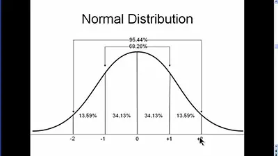
Understanding Normal Distribution

One of the first things that you learn when you start studying statistics is the normal distribution which is also known as the Gaussian distribution or normal bell curve.

Discover the z tables you need here.

normal-distribution

As you can see from the image above, the normal distribution tapers out in both tails and is dense in the middle. 

Imagine that a teacher wants to create a curve based on the exam scores. This means that he will be fitting the scores to the bell curve. When he is filling the chart, the grades will be centered around the mean score (the tallest, central point on the curve, typically signified by the Greek letter μ), which becomes the equivalent of a C grade; the rest of the scores then fall somewhere around this central mean.

The truth is that due to the shape of the curve, most exam scores will be in the middle and fatter portion of the curve. So, we can then state that most students in the class will end up scoring B, C, or D. Why? Because of the thinner tails, fewer students will be found further out from the mean. So, A grades and failing grades will occur less frequently than middle-of-the-road scores.

Understanding z scores, z table, and z transformations.

Practical Example

Now that you already understand the concept of the normal distribution, it’s time to check a practical example. 

Imagine that the average height of a woman in the US is 63.1 inches with a standard deviation of 2.7 inches.

Since height is normally distributed, you can then expect to discover that most American women you will encounter in your life will more likely have a height closer to 5 feet 3 inches than, say, 7 feet. Besides, we can also say that since height is a normally distributed variable, the mean predominates, and extreme values are rare. 

In case you are wondering if this is true or not, just think about how uncommon it is to find giants and dwarves on the street. But just how much more common is the middle-ground than the extremes? 

What to do when you can’t run the ideal analysis.

Probability Distributions

As you probably remember, probability distributions are visual plots of how frequently certain values occur. 

The following is a discrete probability distribution showing the probabilities of every possible roll (from 2 to 12) of two standard 6-sided dice:

Probability-Distributions

If you take a look at the above distribution, you can see that the probability of rolling a 7 (tallest, middle bar) is 1 in 6 (right-hand axis). 

Notice that there’s a difference between this example and the previous one with the heights. After all, our previous variable of height is continuous, because heights can take any value.

The normal distribution is a continuous probability distribution function. So, now we are ready to consider the normal distribution as a continuous probability distribution function. Unlike with discrete probability distributions, where we could find the probability of a single value, for a continuous distribution, we can only find the probability of encountering a range of values.

Discover everything you need to know about standard deviation. 

The 68-95-99.7 Rule

The 68-95-99.7 Rule says that for any normally distributed random variable:

  • 68% of the population will lie within 1 standard deviation, 1σ, of the mean
  • 95% of the population will lie within 2 standard deviations, 2σ, of the mean
  • 99.7% of the population will lie within 3 standard deviations, 3σ, of the mean
The-68-95-99.7-Rule

If you apply this to our previous height example, 68% of all women should have heights within one standard deviation, or 2.7 inches, of the mean. We can calculate this interval as follows:

63.1 ± 2.7 = {60.4,65.8}

Therefore, we expect that 68% of women in the US to have heights between 60.4 and 65.8 inches. The 68-95-99.7 rule is a useful, fast rule of thumb for determining probabilities under the curve. 

Introduction To Probability And Statistics

One of the first questions that most tend to hear when they are learning about probability and statistics is how likely are you to flip a coin and it lands on its edge?

As you can imagine, this lands in the land of probability and statistics. 

Find all the z score values you need. 

What Is Probability?

probability-and-statistics

Simply put, the probability of something is the likelihood of that something to occur. This something, in statistics, is called event or happening. 

Let’s take a look at some examples so you understand the concept completely. 

When you are playing the Dungeons & Dragons game and you need to roll a D20, then you know that getting a 20 is a very good thing most of the time. While everyone says it is incredibly difficult to get a 20, the truth is that it is as difficult to get a 20 as it is to get a 1. But why?

Dungeons-Dragons

What is descriptive statistics?

As we mentioned above, when you are trying to determine the probability (P), this means that you are trying to discover the chance of an event to occur, which is usually written as P(event). 

So, in the case of our D&D dice when you roll it you have these outcomes

S = {1, 2, 3, 4, 5, 6, 7, 8, 9, 10, 11, 12, 13, 14, 15, 16, 17, 18, 19, 20}

This means that the likelihood of rolling a number 1 – 20 is 100% while the likelihood of rolling a 21 is 0%. But the events in between are a little different.

Probability is calculated as the total number of desired outcomes ÷ total number of possible outcomes.

Discover the most common probability distributions.

Taking A Deeper Look At Our Example

We can say that there are 20 total possible events that can happen when you roll a D20. At this point, we’re only interested in getting one outcome – 20. Since it is one of 20 possible outcomes:

P(20) = 1/20 = 0.05

It has the same likelihood of a 1 being rolled:

P(1) = 1/20 = 0.05.

But if you want to roll a number less than 20 is different. After all, this would be:

P(1, 2, 3, 4, 5, 6, 7, 8, 9, 10, 11, 12, 13, 14, 15, 16, 17, 18, 19) = 19/20 = 0.95

We can then say that it is much more likely.

Summing up, rolling a D20 and getting a 20 is just as likely as rolling a 1. However, the reason 20s are so rare is that you are much more likely to roll a number less than 20. 

Learn how to apply the z score in real life. 

Statistics

So, how can you adapt probability to statistics which is all that matters to us? 

understanding-probability-and-statistics

Simply put, statistics is just the application of the laws of probability to real data. If you take the D20 example, this would be when you roll the dice 20 times and collect some data.

When you apply probability to real data, you are trying to determine if the outcome is significantly different from a model that we are generating. For example, the P(20) = 0.05.

Le’s take a closer look at this. 

When you gather your data, you know there are different ways to describe it. The most usual ones are mean, median, and mode. In the case of statistics, you want to see if your actual data conforms to the model. To do this, you have two different options: the classical inference and Bayesian inference.

While classical inference deals with data that have a fixed probability based on the number of cases and events, the Bayesian inference deals with data whose probability is not fixed. That is, the probability is subject to change based on other factors. 

The Most Common Probability Distributions

In statistics, there are many different types of probability distributions. While you tend to read and hear only about norma distribution, the reality is that there are others. Let’s take a closer look at them. 

The Most Common Probability Distributions

#1: Normal Distribution:

probability-distributions

The normal distribution is the most common one. The truth is that the large sum of small random variables tend to be normally distributed. Here are some of the main characteristics of a normal distribution: 

  • The curve of the distribution features a bell shape and is symmetrical.
  • The mean, mode, and median are equal.
  • The total area under the curve is 1 or 100%.
  • Half of the values will be to the left side of the center and the other half to the right. 

Discover more details about the normal distribution.

#2: Bernoulli Distribution:

Bernoulli-Distribution

While the name may scare you, the truth is that this is one of the types of probability distributions that is easier to understand. Simply put, a Bernoulli distribution can only have two possible outcomes. They are 1 (success) and 0 (failure). And then you have a single trial. 

So, the random variable x that has this type of distribution can take value 1 with the probability of success (p) and the value 0 with the probability of failure (q or 1-p). 

Notice that the probabilities in this type of distribution don’t need to be equal. Some examples of Bernoulli distribution include knowing whether it is going to rain or not tomorrow. 

Want to know more about the z score?

#3: Uniform Distribution:

Uniform-Distribution

The basis of an uniform distribution is that the probabilities of getting the different outcomes are equal. One simple example is when you roll a fair die. 

One of the most interesting things about the uniform distribution is its graphical representation. Unlike the normal distribution that resembles a bell, the uniform distribution is rectangular. This is why this distribution is also known as a rectangular distribution. 

Discover how to determine the z score value.

 #4: Binomial Distribution:

Binomial-Distribution

A binomial distribution occurs where there are only two possible outcomes such as win or lose, gain or loss, success or failure. Besides, the probability of success and failure are always the same for all trials. However, the results may be different. Some of the characteristics of the binomial distribution include:

  • There are only two possible outcomes in a trial – success or failure.
  • Each trail is independent.
  • The probability of success and failure is the same for all trials.
  • A total number of n identical trials are conducted. 

 #5: Poisson Distribution:

Poisson-Distribution

Discover more probability distribution types.

The Poisson distribution is applied to cases or situations where events can occur at random points of space and time wherein your interest lies only in the number of occurrences of the event. Some examples that can be modeled by the Poisson distribution include:

  • The number of printing errors are each page of a book.
  • The number of thefts in an area on a day.
  • The number of calls that are made at a call center a day.
  • The number of suicides reported in a specific city.
  • The number of customers arriving at a restaurant in one hour.
  • The number of emergency calls recorded at a hospital in a day.