
Lookup z score in this z table (same as z score table, standard normal distribution table, normal distribution table or z chart). You will also find a z score calculator right after the tables.
Find a value representing the area to the left of a positive Z score in this standard normal distribution table.
Find a value representing the area to the left of a negative Z score in this standard normal distribution table.
Use this Z Score Calculator for quick z value calculation:
| Population Mean: |
The mean (average value) of the population to which the unstandardized value belongs. |
|
| Population Standard Deviation: |
The standard deviation of the population to which the unstandardized value belongs. |
|
| Value: |
The unstandardized raw value for which you want to compute a Z-score. |
|
| Z-Score: | ||
Z Score Lookup Explanation Video
This short video quickly explains how to find area left of a Z score. It also shows the difference between using a left tail and right tail Z table.
Z score Formula
- Z – is a z score
- X – is a raw score
- μ -is a population mean
- σ – is a population standard deviation
What is Z score?
The z-score, which is also known as the standard score, is the number of standard deviations from the mean a data point is. In case you are looking for a more technical definition, then we can say that the z score is a measure of how many standard deviations there are that are above or below the population mean.
One of the things that you need to know about the z score is that when you calculate its mean, the result will always be 0. In addition, the standard deviation or variance will always be in increments of 1.
A z score can be placed on a normal distribution curve. It simply shows the position of the raw score in terms of the distance of this score from the mean when you measure it in standard deviation units. In case you get a positive z score, then you know that the value is above the mean. On the other hand, when you get a negative value, it will be below the mean.
To use a z score, you need to know not only the mean – μ, but also the population standard deviation – σ.
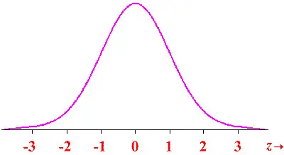
The truth is that a z score also allows you to compare the scores of different variables by standardizing the distribution. The image below shows you the standard normal distribution when the mean is 0 and the standard deviation is 1.
How To Calculate A Z Score?
It is important that you know that while z score isn’t usually calculated by hand (since there is so much data), you can do it as well. To do it, you will need to use the following formula:
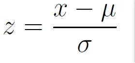
As you can see, you will need to first determine the difference between the raw score and the sample mean, and then divide the result by the sample standard deviation.
Here’s a simple example so that you can easily determine the z score.
Let’s assume that you have a test score of 190. This test has a standard deviation (σ) of 25 and a mean (μ) of 150. Also assuming that you are dealing with a normal distribution, you would need to:
z = (x – μ) / σ
z = (190 – 150) / 25
z = 1.6
As you already know, the z score lets you know how many standard deviations from the mean your score is. So, in this specific example, and considering that we have a positive z score, we can then say that the score you got is 1.6 standard deviations above the mean.
Calculating A Z Score With Excel
As we already mentioned, in the real-life, most z score calculations need to be made using Excel. This doesn’t only allow researchers and statisticians to be faster determining the scores as there will be fewer errors and mistakes. So, here are the steps that you need to take:
Step #1:
The main goal is to find the z score of a specific value. Let’s call it x.
According to the formula we already showed you, you will need to calculate the mean. This is where you should start.
To determine the mean of the sample, you will need to use the AVERAGE formula. In case this is the first time you are doing such calculations, let’s assume that you have a sample that begins at cell A1 and that ends at cell A20. By using the formula =AVERAGE(A1:A20), you will get the average of these numbers.
Step #2:
Now, it is time to calculate the standard deviation of the sample. In order to do this, you will need to use the STDEV.S formula.
Let’s assume again that your scores start in the cell A1 and that they end in the cell A20. So, by using the formula = STDEV.S (A1:A20), you will get the standard deviation of these numbers.
Step #3:
Now, it is finally the time to determine the z score. If you remember, the formula of the z score is (x – mean) / standard deviation. To calculate it, you will need to use an empty cell and type the following formula: = (x – mean) / [standard deviation].
While this can easily be made when you have a small amount of data, it can be a bit tricky when you are using a large population sample. So, it is always preferred to use a slightly different formula to avoid writing all the mean and standard deviation values in the formula by hand. If this is what you prefer, you can then use the following formula: = (A12 – B1) / [C1].
Step #4:
But your work isn’t done yet. The truth is that you will need to calculate the probability for a smaller z score. This means that you will be determining the probability of observing a value less than x, which corresponds to the area under the curve and to the left of x. In this case, you need to use a blank cell and type the formula = NORMSDIST( and input the z-score you calculated).
Step #5:
To determine the probability of the larger z score, which determines the probability of observing a value greater than x and that corresponds to the area under the curve and to the right of x, you will need to use the formula: =1 – NORMSDIST (and input the z-score you calculated). Noticed that this one also needs to be typed in an empty cell.
Interpreting A Z Score
When you finish calculating the z score, it is time to interpret the results. Just as a quick recap, the value of the z score lets you know exactly how many standard deviations you are away from the mean. So,
- If the z score is equal to zero, this means that the z score is equal to the mean.
- If you get a positive z score, this shows you that the raw score is higher than the mean average. So, if, for example, you get a z score equal to +1.3, then you can say that it is 1.3 standard deviations above the mean.
- If you get a negative z score, this shows that the raw score is lower than the mean average. So, if, for example, you get a z score equal to -2.3, then you can say that it is 2.3 standard deviations below the mean.
Some people prefer to interpret results by looking at the standard normal distribution chart and displaying their values there. Notice that the standard normal distribution is also referred to as probability distribution or z score distribution.
Some quick notes about the Standard Normal Distribution:
- The standard normal distribution’s mean is always 0.
- The standard normal distribution’s standard deviation is always 1. This means that one standard deviation of the raw score, no matter what the raw value is, always converts into 1 z score unit.
- The standard normal distribution always features the same shape of the raw score distribution. So, when you have raw scores that are normally distributed, the distribution of z scores will also be normally distributed.
There is also another great use for researchers when they decide to use the standard normal distribution. After all, they can easily determine the probability of getting a score from the distribution or sample.
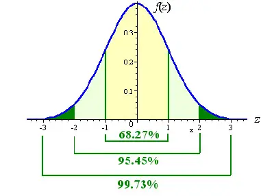
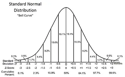
As you can easily see in the image above:
- There is a 68.27% probability of randomly selecting a score between -1 and +1 standard deviations from the mean.
- There is a 95.45%% probability of randomly selecting a score between -1.96 and +1.96 standard deviations from the mean.
- When there is less than a 5% chance of a raw score to be chosen randomly, then we can say that it is a statistically significant result.
#5: Example Of How To Use A Z Score Table (i.e. Standard Normal Table)
A z score table or a standard normal table as it is also referred to is, as we already mentioned above, one very effective way that researchers and statisticians use to determine the probability or area that corresponds to a specific z score. But how can you determine it and put it into practice? Let’s check a practical example so that you can easily understand all the steps involved.
Let’s assume that we randomly select 50 volunteers to take an IQ test. Susan, one of the volunteers, had 74 (x) out of the possible 120 points. We also know that the average score (µ) was 62 and that the standard deviation (σ) was 11. So, what conclusion can we withdraw from here? How well did Susan go on the test compared to the other volunteers?
Step #1: Convert To A Z Score
The first thing that you will need to do is to convert Susan’s IQ test points to a standardized score or to a specific z score that you’re going to use.
So, according to the example provided and using the z score formula that you can find above:
z = (74 – 62) / 11
z = 1.09090909
While we could use this entire z number, it is frequent to round it. So, we are going to say that z = 1.09. And this is the standardized z score that we are going to use.
Step #2: Find The Area That Matches To The Z Score
As soon as you calculate the standardized score, it is now time to look at the area or probability. This is done by checking the Z table. You will need to first look for the two digits on the left side of the Z table which, in this case, is 1.0. Then, as for the remaining number, you will need to look across the table (at the top) and fin the 0.09.
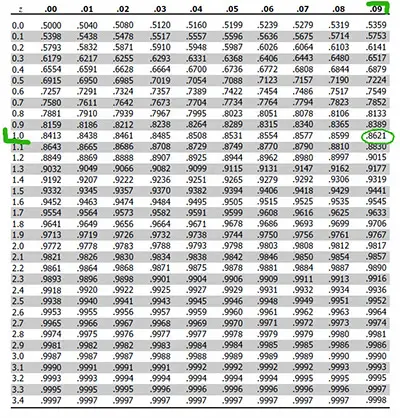
As you will easily see, the corresponding area is 0.8621 which means 86.21%. Notice that on some z score tables, you will see that the area that corresponds to the z score 1.09 is 0.3621. Since the results are different, you may be tempted to think that you’re not doing things right or that you’re looking at the wrong table. This isn’t either. The reality is that there are some z score tables that just show the area to the right and to the left of the mean. So, when you are checking one of these z score tables and you have a positive z score, you will need to sum 0.5 (or 50%) to calculate the area that is to the left of the z score.
So, in this case, it would be 0.5 + 0.3621 = 0.8621, As you can see, both values are identical, no matter if you’re using one z score table or another.
Step #3: Draw A Valid Conclusion
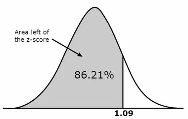
In the above image, you can see the representation of the score that Susan got when compared to the rest of the volunteers when she took the IQ test.
Notice that it is also possible to determine the number of people who Susan outperformed at the test. To do it, you just need to multiply the number of people who took the test (50) by 0.8621:
50 X 0.8621 = 43.1
So, you will need to round the number to 43 since there aren’t partial human beings. Our conclusion is that Susan was able to do better than 43 other volunteers.
Normal Distribution Explained
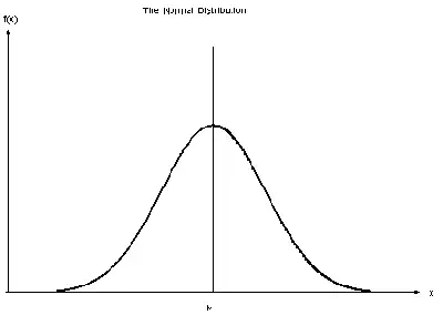
The normal distribution is also known as the Gaussian distribution or even as the standard or normal bell curve.
As you can easily see in the image above, the normal distribution tapers out in both tails and is denser in the middle. This means that all the values are always centered around the mean score which is the central and tallest point of the curve, and is usually known as μ. The rest of the scores fall all into somewhere around it.
If you think about representing the scores of students within the normal distribution, then we can say that most of them would be located in the middle and fatter area of the curve. After all, most students tend to get B, C, and D scores. In what concerns to the thinner tails, they only state that fewer students will fit here. This area refers to students that get A scores.
One of the most important things that you should keep in mind is that the normal distribution is very important especially in inferential statistics. This is due to the fact that there are many random variables that tend to follow this same pattern.
Here’s a practical example.
According to Columbia University Statistics, the average height for a woman in the US is 63.1 inches (or about 5 feet 3 inches), with a standard deviation of 2.7 inches.
One of the things that you need to know about height is that it falls under the normally distributed variables. If you think about it, most people have an average height. It’s uncommon to see someone with 7 feet, for example.
Besides, it is also important to notice that height is continuous. The reality is that you may have a woman with 63.1 inches tall, another one with 63.2 inches and still another with 63.05 inches. Basically, there are no restrictions. This is why we can say that the variable is continuous.
Notice that with the normal distribution and continuous variables as it is the case of height, you can’t answer the question “What is the probability that a random woman in New York City is 63.1 inches tall?”. However, you can answer a different one: “What’s the probability that a random woman in New York City is between 60.4 and 63.8 inches tall?”
The 68-95-99.7 Rule
This is a very simple rule that shows that for any normally distributed random variable:
- 68% of the population will lie within 1 standard deviation, 1σ, of the mean.
- 95% of the population will lie within 2 standard deviations, 2σ, of the mean.
- 99.7% of the population will lie within 3 standard deviations, 3σ, of the mean.
Using this rule in our height example, the mean height of women in the United Staes is 63.1 inches. Besides, we also know that the standard deviation is 2.7 inches.
According to the 68-95-99.7 rule, we can say that 68% of all women have heights within 1 standard deviation or are 2.7 inches of the mean:
63.1 ± 2.7 = {60.4,65.8}
As you can see, we can say that 68% of women in the United States have heights between 60.4 and 65.8 inches.
Z Score PDF
To ensure that you can easily determine the value of the z score, we are providing you with a Z Score table in PDF. This way, you can easily open it or even download it.
Z Table Two Tailed Normal Curve: How To Find The Area
While you probably already heard about a two tailed normal curve, you may not know what it is or what it is used for. The truth is that a two tailed normal curve is a curve as the name says but there is an area in each one of the two tails. So, to determine this area, you will need to know how to read a z score table.
As we already mentioned, z score tables are lists of percentages. You need to know that the total area under the curve is 100% and the z score tale shoes areas as a fraction of this percentage.
Here are the steps that you need to take:
Step #1: Look In The Z Table For one of the z values by finding the intersection
Let’s say that you want to find the area in the left tail of z = -0.46. In this case, you will need to search for the 0.4 on the left side and then look at the top row to and search for the 0.06. The intersection of the column with the line gives you 0.1772.
Step #2: Subtract The Z Value From 0.50
The next thing that you will need to do is to subtract the z value that you just found (0.1772) from 0.50:
0.50 – 0.1772 = 0.3228.
Step #3: Repeat The Process
While you have only looked at the left tail until now, you will need to repeat the steps 1 and 2 for the right tail as well.
One of the things that you need to know is that, in most cases, the two tails are symmetrical. Let’s assume that this is the case and that you also get the 0.3228 as a result.
Step #4: Add Both Z Values Together:
In the two tailed normal curve, you will need to add the value that you got for the left tail with the one that you got for the right tail:
0.3228 + 0.3228 = 0.6456
The Bell Curve
The Bell curve is nothing more and nothing else than the normal distribution that we already mentioned above. It refers to a distribution that occurs naturally in many situations.
While you may have never heard about the Bell Curve, you probably already saw it in action. After all, the Bell curve is often seen in tests such as the GRE or SAT. Considering that most students score the average (C), there are less who score a B or a D. The percentage will be even smaller if you take into account scores such as A or F. And this create a distribution that seems like a bell and this is where the name comes from.
One of the things that you need to know about the Bell curve is that it is symmetrical and that half of the data will fall into the right side of the mean and the other half into the left side of the mean.
There are a lot of groups that follow this pattern and this is why the Bell curve is very used. Some of the examples where you can see it may be related to business, government bodies such as the FDA, statistics, IQ scores, blood pressure, heights of people, salaries, measurement errors, points on a test, among many others.